Quickstart/Cheat-Sheet
Warning
This is documentation for an early access release of pyglotaran, certain aspects of how it works (as demonstrated in this quickstart) may be subjected to changes in future 0.x releases of the software. Please consult the pyglotaran readme to learn more on what this means.
To start using pyglotaran in your project, you have to import it first. In addition we need to import some extra components for later use.
In [1]: import glotaran as gta

In [2]: from glotaran.analysis.optimize import optimize

In [3]: from glotaran.analysis.scheme import Scheme
Let us get some data to analyze:
In [4]: from glotaran.examples.sequential import dataset

In [5]: dataset
Out[5]:
<xarray.Dataset>
Dimensions:   (spectral: 72, time: 2100)
Coordinates:
  * time      (time) float64 -1.0 -0.99 -0.98 -0.97 ... 19.96 19.97 19.98 19.99
  * spectral  (spectral) float64 600.0 601.4 602.8 604.2 ... 696.6 698.0 699.4
Data variables:
    data      (time, spectral) float64 0.01551 0.02087 0.001702 ... 1.714 1.538
Like all data in pyglotaran, the dataset is a xarray.Dataset.
You can find more information about the xarray library the xarray hompage.
The loaded dataset is a simulated sequential model.
To plot our data, we must first import matplotlib.
In [6]: import matplotlib.pyplot as plt
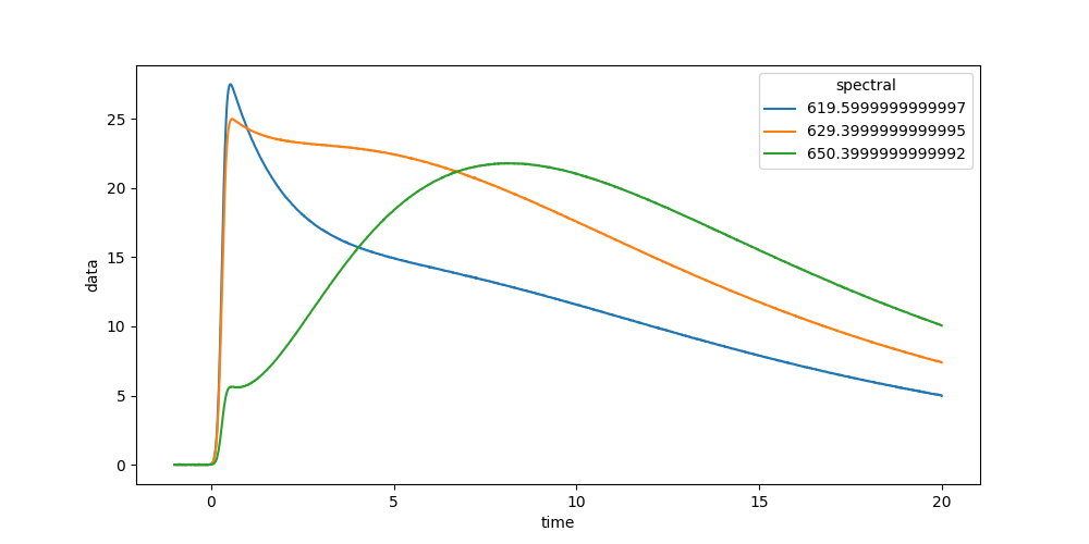
Now we can plot some time traces.
In [7]: plot_data = dataset.data.sel(spectral=[620, 630, 650], method='nearest')

In [8]: plot_data.plot.line(x='time', aspect=2, size=5);
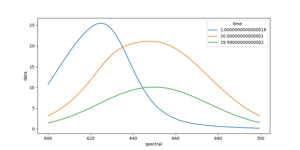
We can also plot spectra at different times.
In [9]: plot_data = dataset.data.sel(time=[1, 10, 20], method='nearest')

In [10]: plot_data.plot.line(x='spectral', aspect=2, size=5);
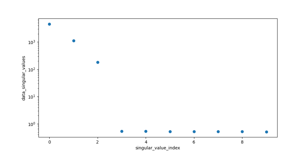
To get an idea about how to model your data, you should inspect the singular value decomposition. Pyglotaran has a function to calculate it (among other things).
In [11]: dataset = gta.io.prepare_time_trace_dataset(dataset)

In [12]: dataset
Out[12]:
<xarray.Dataset>
Dimensions:                      (left_singular_value_index: 72, right_singular_value_index: 72, singular_value_index: 72, spectral: 72, time: 2100)
Coordinates:
  * time                         (time) float64 -1.0 -0.99 -0.98 ... 19.98 19.99
  * spectral                     (spectral) float64 600.0 601.4 ... 698.0 699.4
Dimensions without coordinates: left_singular_value_index, right_singular_value_index, singular_value_index
Data variables:
    data                         (time, spectral) float64 0.01551 ... 1.538
    data_left_singular_vectors   (time, left_singular_value_index) float64 -8...
    data_singular_values         (singular_value_index) float64 4.62e+03 ... ...
    data_right_singular_vectors  (right_singular_value_index, spectral) float64 ...
First, take a look at the first 10 singular values:
In [13]: plot_data = dataset.data_singular_values.sel(singular_value_index=range(0, 10))

In [14]: plot_data.plot(yscale='log', marker='o', linewidth=0, aspect=2, size=5);
To analyze our data, we need to create a model. Create a file called model.yml
in your working directory and fill it with the following:
type: kinetic-spectrum

initial_concentration:
  input:
    compartments: [s1, s2, s3]
    parameters: [input.1, input.0, input.0]

k_matrix:
  k1:
    matrix:
      (s2, s1): kinetic.1
      (s3, s2): kinetic.2
      (s3, s3): kinetic.3

megacomplex:
  m1:
    k_matrix: [k1]

irf:
  irf1:
    type: gaussian
    center: irf.center
    width: irf.width

dataset:
  dataset1:
    initial_concentration: input
    megacomplex: [m1]
    irf: irf1
Now you can load the model file.
In [15]: model = gta.read_model_from_yaml_file('model.yml')
You can check your model for problems with model.validate.
In [16]: print(model.validate())
Your model is valid.
Now define some starting parameters. Create a file called parameters.yml with
the following content.
input:
  - ['1', 1, {'vary': False, 'non-negative': False}]
  - ['0', 0, {'vary': False, 'non-negative': False}]

kinetic: [
     0.5,
     0.3,
     0.1,
]

irf:
  - ['center', 0.3]
  - ['width', 0.1]
In [17]: parameters = gta.read_parameters_from_yaml_file('parameters.yml')
You can model.validate also to check for missing parameters.
In [18]: print(model.validate(parameters=parameters))
Your model is valid.
Since not all problems in the model can be detected automatically it is wise to visually inspect the model. For this purpose, you can just print the model.
In [19]: print(model)
# Model

_Type_: kinetic-spectrum

## Initial Concentration

* **input**:
  * *Label*: input
  * *Compartments*: ['s1', 's2', 's3']
  * *Parameters*: [input.1, input.0, input.0]
  * *Exclude From Normalize*: []

## K Matrix

* **k1**:
  * *Label*: k1
  * *Matrix*:
    * *('s2', 's1')*: kinetic.1
    * *('s3', 's2')*: kinetic.2
    * *('s3', 's3')*: kinetic.3


## Irf

* **irf1** (gaussian):
  * *Label*: irf1
  * *Type*: gaussian
  * *Center*: irf.center
  * *Width*: irf.width
  * *Normalize*: False
  * *Backsweep*: False

## Dataset

* **dataset1**:
  * *Label*: dataset1
  * *Megacomplex*: ['m1']
  * *Initial Concentration*: input
  * *Irf*: irf1

## Megacomplex

* **m1**:
  * *Label*: m1
  * *K Matrix*: ['k1']
The same way you should inspect your parameters.
In [20]: print(parameters)
* __None__:
  * __input__:
    * __1__: _Value_: 1.0, _StdErr_: 0.0, _Min_: -inf, _Max_: inf, _Vary_: False, _Non-Negative_: False, _Expr_: None
    * __0__: _Value_: 0.0, _StdErr_: 0.0, _Min_: -inf, _Max_: inf, _Vary_: False, _Non-Negative_: False, _Expr_: None
  * __kinetic__:
    * __1__: _Value_: 0.5, _StdErr_: 0.0, _Min_: -inf, _Max_: inf, _Vary_: True, _Non-Negative_: False, _Expr_: None
    * __2__: _Value_: 0.3, _StdErr_: 0.0, _Min_: -inf, _Max_: inf, _Vary_: True, _Non-Negative_: False, _Expr_: None
    * __3__: _Value_: 0.1, _StdErr_: 0.0, _Min_: -inf, _Max_: inf, _Vary_: True, _Non-Negative_: False, _Expr_: None
  * __irf__:
    * __center__: _Value_: 0.3, _StdErr_: 0.0, _Min_: -inf, _Max_: inf, _Vary_: True, _Non-Negative_: False, _Expr_: None
    * __width__: _Value_: 0.1, _StdErr_: 0.0, _Min_: -inf, _Max_: inf, _Vary_: True, _Non-Negative_: False, _Expr_: None
Now we have everything together to optimize our parameters. First we import optimize.
In [21]: scheme = Scheme(model, parameters, {'dataset1': dataset})

In [22]: result = optimize(scheme)
   Iteration     Total nfev        Cost      Cost reduction    Step norm     Optimality
       0              1         7.5381e+00                                    3.74e+01
       1              2         7.5377e+00      4.62e-04       1.02e-04       3.28e-01
       2              3         7.5377e+00      9.13e-10       3.48e-08       3.49e-06
`ftol` termination condition is satisfied.
Function evaluations 3, initial cost 7.5381e+00, final cost 7.5377e+00, first-order optimality 3.49e-06.

In [23]: print(result)
Optimization Result            |            |
-------------------------------|------------|
 Number of residual evaluation |          3 |
           Number of variables |          5 |
          Number of datapoints |     151200 |
            Degrees of freedom |     151195 |
                    Chi Square |   1.51e+01 |
            Reduced Chi Square |   9.97e-05 |
 Root Mean Square Error (RMSE) |   9.99e-03 |


In [24]: print(result.optimized_parameters)
* __None__:
  * __input__:
    * __1__: _Value_: 1.0, _StdErr_: 0.0, _Min_: -inf, _Max_: inf, _Vary_: False, _Non-Negative_: False, _Expr_: None
    * __0__: _Value_: 0.0, _StdErr_: 0.0, _Min_: -inf, _Max_: inf, _Vary_: False, _Non-Negative_: False, _Expr_: None
  * __kinetic__:
    * __1__: _Value_: 0.4999391441068187, _StdErr_: 0.007261698651628417, _Min_: -inf, _Max_: inf, _Vary_: True, _Non-Negative_: False, _Expr_: None
    * __2__: _Value_: 0.30008042937966384, _StdErr_: 0.0041961923515427, _Min_: -inf, _Max_: inf, _Vary_: True, _Non-Negative_: False, _Expr_: None
    * __3__: _Value_: 0.0999874440333988, _StdErr_: 0.0004778304467913974, _Min_: -inf, _Max_: inf, _Vary_: True, _Non-Negative_: False, _Expr_: None
  * __irf__:
    * __center__: _Value_: 0.30000199460726046, _StdErr_: 0.0005010729238540931, _Min_: -inf, _Max_: inf, _Vary_: True, _Non-Negative_: False, _Expr_: None
    * __width__: _Value_: 0.09999158675249081, _StdErr_: 0.0006703684374783712, _Min_: -inf, _Max_: inf, _Vary_: True, _Non-Negative_: False, _Expr_: None
You can get the resulting data for your dataset with result.get_dataset.
In [25]: result_dataset = result.get_dataset('dataset1')

In [26]: result_dataset
Out[26]:
<xarray.Dataset>
Dimensions:                                   (clp_label: 3, component: 3, from_species: 3, left_singular_value_index: 72, right_singular_value_index: 72, singular_value_index: 72, species: 3, spectral: 72, time: 2100, to_species: 3)
Coordinates:
  * time                                      (time) float64 -1.0 ... 19.99
  * spectral                                  (spectral) float64 600.0 ... 699.4
  * clp_label                                 (clp_label) <U2 's1' 's2' 's3'
  * species                                   (species) <U2 's1' 's2' 's3'
    rate                                      (component) float64 -0.4999 ......
    lifetime                                  (component) float64 -2.0 ... -10.0
  * to_species                                (to_species) <U2 's1' 's2' 's3'
  * from_species                              (from_species) <U2 's1' 's2' 's3'
Dimensions without coordinates: component, left_singular_value_index, right_singular_value_index, singular_value_index
Data variables: (12/24)
    data                                      (time, spectral) float64 0.0155...
    data_left_singular_vectors                (time, left_singular_value_index) float64 ...
    data_singular_values                      (singular_value_index) float64 ...
    data_right_singular_vectors               (right_singular_value_index, spectral) float64 ...
    matrix                                    (time, clp_label) float64 6.006...
    clp                                       (spectral, clp_label) float64 1...
    ...                                        ...
    a_matrix                                  (component, species) float64 1....
    k_matrix                                  (to_species, from_species) float64 ...
    k_matrix_reduced                          (to_species, from_species) float64 ...
    irf_center                                float64 0.3
    irf_width                                 float64 0.09999
    irf                                       (time) float64 1.976e-37 ... 0.0
Attributes:
    root_mean_square_error:           0.009985218742264433
    weighted_root_mean_square_error:  0.009985218742264433
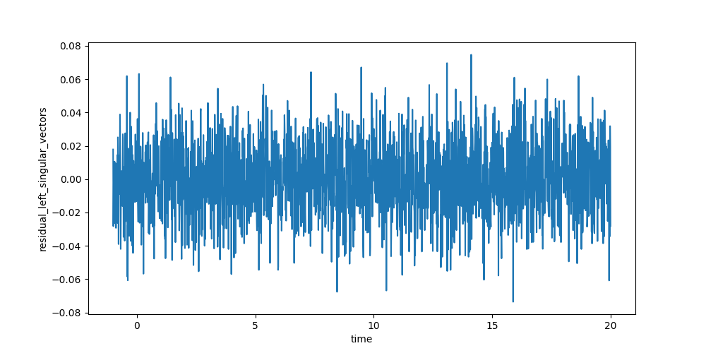
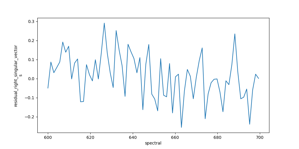
The resulting data can be visualized the same way as the dataset. To judge the quality of the fit, you should look at first left and right singular vectors of the residual.
In [27]: plot_data = result_dataset.residual_left_singular_vectors.sel(left_singular_value_index=0)

In [28]: plot_data.plot.line(x='time', aspect=2, size=5);
In [29]: plot_data = result_dataset.residual_right_singular_vectors.sel(right_singular_value_index=0)

In [30]: plot_data.plot.line(x='spectral', aspect=2, size=5);
Finally, you can save your result.
In [31]: result_dataset.to_netcdf('dataset1.nc')